I was interested in taking a look at the standings of my fantasy baseball league to see which teams acutally belonged in their respective ranking, as indicated by their expected roto ranking. I was having a hard time extracting the data from the ESPN Fantasy site into R using the XML package. My problems may have occurred due to the fact that ESPN fantasy baseball leagues are password-protected. Fortunately, I found a way to bypass these data scraping problems - the datapasta package.
1. Load Packages
library(tidyverse)
library(datapasta)
library(backports)
library(reshape2)
library(ggthemes)
2. Data Extraction
The datapasta package is really convenient because it allows you to copy-paste tables from the internet straight into R. The table will appear in R as a tribble (or transported tibble), which is a nice readable format. I used a custom keyboard shortcut for the tribble paste, as the package authors recommend. After copy-tribble pasting my league’s fantasy standings into R, the cursor shows:
df <- tibble::tribble(
  ~V1,                             ~V2, ~V3,  ~V4,  ~V5,  ~V6,  ~V7,   ~V8,   ~V9, ~V10,  ~V11, ~V12, ~V13, ~V14,  ~V15,  ~V16, ~V17, ~V18,
   1L,             "The Doge of Kyoto",  NA, 882L, 267L, 811L,  91L, 0.2697, 0.8297,   NA, 1689L, 136L, 114L,  72L, 3.754, 1.214,   NA,  96L,
   2L,                  "Judge Mental",  NA, 889L, 281L, 861L,  97L, 0.2838, 0.8631,   NA, 1545L, 119L,  96L,  55L, 3.825, 1.261,   NA,  90L,
   3L,   "Giancarlo's Golden Sombrero",  NA, 858L, 243L, 797L, 145L, 0.2805, 0.8205,   NA, 1388L, 110L,  88L,  80L, 4.104, 1.288,   NA,  86L,
   4L,         "Mark Mangino Auriemma",  NA, 832L, 239L, 792L,  82L, 0.2647, 0.8029,   NA, 1538L, 123L, 115L,  92L, 3.829, 1.282,   NA,  94L,
   5L,              "Harper's Fairies",  NA, 842L, 239L, 797L,  93L, 0.2612, 0.8006,   NA, 1538L, 103L,  97L, 131L, 3.822, 1.234,   NA, 139L,
   6L,    "PutMy Dickerson In her BOX",  NA, 720L, 207L, 680L, 103L, 0.2562, 0.7804,   NA, 1481L, 107L,  96L, 118L, 3.928, 1.247,   NA,  67L,
   7L,             "The Fall of Janet",  NA, 814L, 259L, 852L,  89L, 0.2645, 0.8226,   NA, 1329L, 111L, 101L,  84L, 3.902, 1.255,   NA,  68L,
   8L, "These guys all Doo(too)little",  NA, 704L, 241L, 716L,  59L, 0.2738, 0.8167,   NA, 1468L, 112L,  83L,  84L, 4.266, 1.346,   NA,  35L,
   9L,                "Hakuna Moncada",  NA, 747L, 208L, 698L, 146L, 0.2705, 0.7873,   NA, 1186L,  94L,  85L,  38L, 4.495, 1.334,   NA, 122L,
  10L,             "Colossus of Trout",  NA, 770L, 214L, 672L,  94L, 0.2598, 0.7926,   NA, 1357L, 114L,  93L,  42L, 4.269, 1.256,   NA,  26L,
  11L,                "Captain inSano",  NA, 685L, 204L, 738L,  65L, 0.2666, 0.767,   NA, 1177L, 104L,  83L,  52L, 4.167, 1.299,   NA,  40L,
  12L,               "Tanking Machine",  NA, 786L, 220L, 738L,  49L, 0.286, 0.8333,   NA,  906L,  72L,  60L,  88L, 3.832, 1.222,   NA,   9L
  )
Besides, the extra “blank” columns, this dataset is perfect.
3. Obtaining the Roto Ranks
Our league is setup such that each week there are 12 categories (6 pitching, 6 hitting) available to win. A team’s ranking is based on the cumulative win-loss-tie record of these weekly matchups. On the other hand, a roto ranking does not take into account weekly performance, only overall performance. In our league with 12 teams, if you performed the best in a category, you would score a 1 for that category. If you performed the worst in that cateogry, you would score a 12. For each team, these scores are summed for the 12 categories and the teams would be ranked lowest to highest.
First, every category (except for ERA and WHIP) needs to be ranked in descending order (high values correspond to lower ranks). ERA and WHIP are unique in that lower values win you the category.
ranked <-
  df %>% mutate(
    R = rank(-R),
    HR = rank(-HR),
    RBI = rank(-RBI),
    SB = rank(-SB),
    AVG = rank(-AVG),
    OPS = rank(-OPS),
    K = rank(-K),
    QS = rank(-QS),
    W = rank(-W),
    SV = rank(-SV),
    ERA = rank(ERA),
    WHIP = rank(WHIP))
The apply function will be used to sum over the rows (i.e. the teams). Lastly, these row totals will be ranked in ascending order.
ranked$ranktotal <- apply(ranked[, 3:15], 1, sum)

ranked$FinalROTOrank <- rank(ranked$ranktotal)
We’ll examine these roto rankings in the next section.
4. Plotting the Results
To visualize the final roto rankings, we will use an ordered and grouped bar chart.
Preparing the data:
plotdata <- ranked[, c(2, 1, 17)]
plotdata <- melt(plotdata, id.vars="team")
plotdata$team <- sub("^(\\S*\\s+\\S+).*", "\\1", plotdata$team)
plotdata <- rename(plotdata, Type = variable)

plotdata <- data.frame(lapply(plotdata, function(x) {gsub("FinalROTOrank", "Expected Roto Rank", x)}), stringsAsFactors=FALSE)
plotdata <- data.frame(lapply(plotdata, function(x) {gsub("rank", "Final Rank", x)}), stringsAsFactors=FALSE)
plotdata$team <- factor(plotdata$team, levels = unique(plotdata$team))
plotdata$Type <- factor(plotdata$Type, levels = c('Final Rank', 'Expected Roto Rank'))
plotdata$value <- as.numeric(plotdata$value)

levels(plotdata$team) <- gsub(" ", "\n", levels(plotdata$team))
Plotting the data:
ggplot(plotdata, aes(fill = Type, x = team, y = value)) +
  theme_fivethirtyeight() +
  geom_bar(position="dodge", stat="identity") +
  labs(title="Regular Season Final Rank Vs Expected Roto Rank",
       subtitle="Ordered & Grouped Bar Chart") +
  scale_y_continuous(breaks = 1:12)
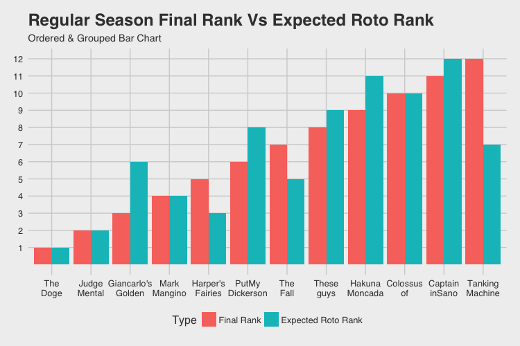
5. Conclusions
In comparing the expected roto rank to the actual regular season rank, first and second place stayed firm in their respective positions. Team Dickerson, who squeaked into the playoffs and ended up winning the championship, would not have been a top-6 team in the roto rankings, suggesting that this owner was lucky to make the playoffs. The 12th place team, Tanking Machine, would have actually finished as a 7th place team in roto, suggesting that this owner was not nearly as bad as his regular season record indicates.