Overview
This tutorial will demonstrate how to adjust for an uncontrolled confounder. First, generate a dataset of 100,000 rows with the following binary variables:
- X = Exposure (1 = exposed, 0 = not exposed)
- Y = Outcome (1 = outcome, 0 = no outcome)
- C = Known Confounder (1 = present, 0 = absent)
- U = Uncontrolled Confounder (1 = present, 0 = absent)
set.seed(1234)
n <- 100000

c <- rbinom(n, 1, 0.5)
u <- rbinom(n, 1, 0.5)
x  <- rbinom(n, 1, plogis(-0.5 + 0.5 * C + 1.5 * U))
y  <- rbinom(n, 1, plogis(-0.5 + log(2) * X + 0.5 * C + 1.5 * U))

df <- data.frame(X = x, Y = y, C = c, U = u)
rm(c, u, x, y)
This data reflects the following causal relationships:

From this dataset note that P(Y=1|X=1, C=c, U=u) / P(Y=1|X=0, C=c, U=u) should equal expit(log(2)). Therefore, odds(Y=1|X=1, C=c, U=u) / odds(Y=1|X=0, C=c, U=u) = ORYX = exp(log(2)) = 2.
Compare the biased (confounded) model to the bias-free model.
nobias_model <- glm(Y ~ X + C + U,
                    family = binomial(link = "logit"),
                    data = df)
exp(coef(nobias_model)[2])
c(exp(coef(nobias_model)[2]) + summary(nobias_model)$coef[2, 2] * qnorm(.025)),
  exp(coef(nobias_model)[2]) + summary(nobias_model)$coef[2, 2] * qnorm(.975)))
ORYX = 2.02 (1.96, 2.09)
This estimate corresponds to the odds ratio we would expect based off of the derivation of Y.
biased_model <- glm(Y ~ X + C,
                    family = binomial(link = "logit"),
                    data = df)
exp(coef(biased_model)[2])
c(exp(coef(biased_model)[2] + summary(biased_model)$coef[2, 2] * qnorm(.025)),
  exp(coef(biased_model)[2] + summary(biased_model)$coef[2, 2] * qnorm(.975)))
ORYX = 3.11 (3.03, 3.20)
The odds ratio of the effect of X on Y increases from ~2 to ~3 when adjustment for the confounder U is absent in the model. In a perfect world, an investigator would simply make sure to control for all confounding variables in the analysis. However, it may not be feasible or possible to collect data on certain variables. This bias analysis will allow for the adjustment of uncontrolled confounders even when data for U is unavailable. We will instead rely on assumptions of how the exposure, outcome, and known confounder(s) affect the unknown confounder. These assumptions are quantified in bias parameters used in the analysis. Using these bias parameters, we can predict the probability of U for each observation and use the probabilities for bias adjustment by either imputing the value of U or by using a regression weighting approach.
Normally, the values of the bias parameters are obtained externally from the literature or from an internal validation sub-study. However, for this proof of concept, we can obtain the exact values of the parameters. We will perform the final regression of Y on X as if we don’t have data on U. Since we have the values of U in our data we can model how U is affected by X, Y, and C to obtain accurate bias parameters.
u_model <- glm(U ~ X + Y + C,
               family = binomial(link = "logit"),
               data = df)
summary(u_model)
These parameters can be interpreted as follows:
- Intercept: log[odds(U=1|X=0, C=0, Y=0)]
- X coefficient: log[odds(U=1|X=1, C=0, Y=0)] / log[odds(U=1|X=0, C=0, Y=0)] i.e. the log odds ratio denoting the amount by which the log odds of U=1 changes for every 1 unit increase in X among the C=0, Y=0 subgroup.
- Y coefficient: log[odds(U=1|X=0, C=0, Y=1)] / log[odds(U=1|X=0, C=0, Y=0)]
- C coefficient: log[odds(U=1|X=0, C=1, Y=0)] / log[odds(U=1|X=0, C=0, Y=0)]
Now that values for the bias parameters have been obtained, we’ll use these values to perform the bias adjustment with two different approaches. In both cases, we’ll build the analysis within a function for quick reiteration. Bootstrapping will be used in order to obtain a confidence interval for the ORYX estimate.
1. Weighting Approach
The steps for the weighting approach are as follows:
- Sample with replacement from the dataset to get the bootstrap sample.
- Predict the probability of U by combining the bias parameters with the data for X, Y, and C via the inverse logit transformation.
- Duplicate the bootstrap sample and merge these two copies.
- In the combined data, assign variable Ubar, which equals 1 in the first data copy and equals 0 in the second data copy.
- Create variable u_weight, which equals the probability of U=1 in the first copy and equals 1 minus the probability of U=1 in the second copy.
- With the combined dataset, model the weighted logistic outcome regression [P(Y=1)| X, C, Ubar]. The weights used in the regression come from u_weight.
- Save the exponentiated X coefficient, corresponding to the odds ratio effect estimate of X on Y.
- Repeat the above steps with a new bootstrap sample.
- With the resulting vector of odds ratio estimates, obtain the final estimate and confidence interval from the median and 2.5, 97.5 quantiles, respectively.
adjust_uc_wgt_loop <- function(
  coef_0, coef_x, coef_c, coef_y, nreps, plot = FALSE
) {
  est <- vector()
  for (i in 1:nreps){
    bdf <- df[sample(seq_len(n), n, replace = TRUE), ]
    prob_u <- plogis(coef_0 + coef_x * bdf$X + coef_c * bdf$C + coef_y * bdf$Y)
    combined <- dplyr::bind_rows(bdf, bdf)
    combined$Ubar <- rep(c(1, 0), each = n)
    combined$u_weight <- c(prob_u, 1 - prob_u)
    final_model <- glm(Y ~ X + C + Ubar, family = binomial(link = "logit"),
                       data = combined, weights = combined$u_weight)
    est[i] <- exp(coef(final_model)[2])
  }
  out <- list(
    estimate = round(median(est), 2),
    ci = round(quantile(est, c(.025, .975)), 2)
  )
  if (plot) {
    out$hist <- hist(exp(est))
  }
  return(out)
}
2. Imputation Approach
The steps for the imputation approach are as follows:
- Sample with replacement from the dataset to get the bootstrap sample.
- Predict the probability of U by combining the bias parameters with the data for X, Y, and C via the inverse logit transformation.
- Impute the value of the uncontrolled confounder, Upred, across Bernoulli trials where the probability of each trial corresponds to the probability of U determined above.
- With the bootstrap sample, model the logistic outcome regression [P(Y=1)| X, C, Upred].
- Save the exponentiated X coefficient, corresponding to the odds ratio effect estimate of X on Y.
- Repeat the above steps with a new bootstrap sample.
- With the resulting vector of odds ratio estimates, obtain the final estimate and confidence interval from the median and 2.5, 97.5 quantiles, respectively.
adjust_uc_imp_loop <- function(
  coef_0, coef_x, coef_c, coef_y, nreps, plot = FALSE
) {
  est <- vector()
  for (i in 1:nreps){
    bdf <- df[sample(seq_len(n), n, replace = TRUE), ]
    bdf$Upred <- rbinom(n, 1, plogis(coef_0 + coef_x * bdf$X +
                                       coef_c * bdf$C + coef_y * bdf$Y))
    final_model <- glm(Y ~ X + C + Upred,
                       family = binomial(link = "logit"),
                       data = bdf)
    est[i] <- exp(coef(final_model)[2])
  }
  out <- list(
    estimate = round(median(est), 2),
    ci = round(quantile(est, c(.025, .975)), 2)
  )
  if (plot) {
    out$hist <- hist(exp(est))
  }
  return(out)
}
Evaluate
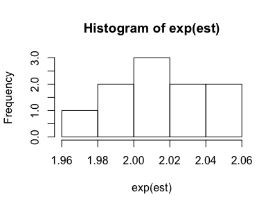
We can run the analysis using different values of the bias parameters. When we use the known, correct values for the bias parameters that we obtained earlier, we obtain ORYX = 2.03 (1.98, 2.07), representing the bias-adjusted effect estimate we expect based on the derivation of the data.
set.seed(1234)
correct_results <- adjust_uc_wgt_loop(
  coef_0 = coef(u_model)[1],
  coef_x = coef(u_model)[2],
  coef_c = coef(u_model)[3],
  coef_y = coef(u_model)[4],
  nreps = 10
)

correct_results$estimate
correct_results$ci
The output can also include a histogram showing the distribution of the ORYX estimates from each bootstrap sample. We can analyze this plot to see how well the odds ratios converge.
If instead we use bias parameters that are each double the correct value, we obtain ORYX = 0.81 (0.79, 0.82), an incorrect estimate of effect.
library(dplyr)

set.seed(1234)
incorrect_results <- adjust_uc_wgt_loop(
  coef_0 = coef(u_model)[1] * 2,
  coef_x = coef(u_model)[2] * 2,
  coef_c = coef(u_model)[3] * 2,
  coef_y = coef(u_model)[4] * 2,
  nreps = 10
)

incorrect_results$estimate
incorrect_results$ci
You can find the full code for this analysis here.