Adjustment for Uncontrolled Confounding

Overview

Observational studies often lack data on important confounders. When an unmeasured variable U confounds the exposure–outcome relationship, standard regression cannot remove the bias—and as we will see, omitting U can materially inflate the estimated effect. Quantitative bias analysis (QBA) makes that systematic uncertainty explicit by encoding assumptions about U in bias parameters and using them to obtain a bias-adjusted estimate.

Here we work through a probabilistic variant: specify a model for P(U | X, Y, C), use those parameters to predict U (or its probability) for each row, and propagate uncertainty with bootstrap resampling. Instead of scanning a table of scenarios, we embed the bias model in the analysis and examine how the adjusted estimate changes when the parameter inputs are correct or wrong.

We simulate data with a known causal effect, show the bias when U is unobserved, and implement two adjustment methods: regression weighting and stochastic imputation.

First, generate a dataset of 100,000 rows with the following binary variables:

X = Exposure (1 = exposed, 0 = not exposed)
Y = Outcome (1 = outcome, 0 = no outcome)
C = Known Confounder (1 = present, 0 = absent)
U = Uncontrolled Confounder (1 = present, 0 = absent)

library(dplyr)

set.seed(1234)
n <- 100000

c <- rbinom(n, 1, 0.5)
u <- rbinom(n, 1, 0.5)
x  <- rbinom(n, 1, plogis(-0.5 + 0.5 * C + 1.5 * U))
y  <- rbinom(n, 1, plogis(-0.5 + log(2) * X + 0.5 * C + 1.5 * U))

df <- data.frame(X = x, Y = y, C = c, U = u)
rm(c, u, x, y)

This data reflects the following causal relationships:

uc_dag

From this dataset note that P(Y=1|X=1, C=c, U=u) / P(Y=1|X=0, C=c, U=u) should equal expit(log(2)). Therefore, odds(Y=1|X=1, C=c, U=u) / odds(Y=1|X=0, C=c, U=u) = OR_YX = exp(log(2)) = 2.

Compare the biased (confounded) model to the bias-free model.

nobias_model <- glm(Y ~ X + C + U,
                    family = binomial(link = "logit"),
                    data = df)
exp(coef(nobias_model)[2])
c(exp(coef(nobias_model)[2]) + summary(nobias_model)$coef[2, 2] * qnorm(.025)),
  exp(coef(nobias_model)[2]) + summary(nobias_model)$coef[2, 2] * qnorm(.975)))

OR_YX = 2.02 (1.96, 2.09)

This estimate corresponds to the odds ratio we would expect based off of the derivation of Y.

biased_model <- glm(Y ~ X + C,
                    family = binomial(link = "logit"),
                    data = df)
exp(coef(biased_model)[2])
c(exp(coef(biased_model)[2] + summary(biased_model)$coef[2, 2] * qnorm(.025)),
  exp(coef(biased_model)[2] + summary(biased_model)$coef[2, 2] * qnorm(.975)))

OR_YX = 3.11 (3.03, 3.20)

The odds ratio increases from ~2 to ~3 when U is omitted, a concrete illustration of uncontrolled confounding. The sections below specify the assumptions needed to adjust for U without observing it, obtain bias parameters, and apply two correction methods. Note that we’ll be assuming all base assumptions for causal identification (e.g., positivity) are already present.

Assumptions for bias adjustment

The adjusted estimate depends on a bias model that describes how the unmeasured confounder U relates to the variables we do observe. Here we use a logistic model for the probability that U = 1:

P(U = 1 | X, Y, C) = expit(β₀ + β_X X + β_Y Y + β_C C)

The intercept and coefficients are bias parameters. They are not identified from the selected sample alone; they must be supplied from external sources.

Why include Y? The model includes Y not because we assume Y causes U, but because Y is observed and may carry information about U once X and C are held fixed. In the DAG above, U sits on back-door paths to both X and Y, and X affects Y, so U and Y are associated in the observed data even when U does not causally depend on Y. Specifying P(U | X, Y, C) is a modeling choice: it uses all available information to predict U for each row before re-fitting the outcome model.

Where parameters come from in practice. Bias parameters are usually set from prior literature, a validation or surrogate substudy, meta-analytic estimates, or structured expert judgment—not by regressing on the true U, which is unknown by definition. Ranges or probability distributions over parameters can be used to reflect uncertainty; the doubled-parameter example later shows how sensitive the adjusted estimate is to misspecification.

Proof of concept in this simulation. Because we generated U, we can fit glm(U ~ X + Y + C) as an oracle exercise: it recovers the conditional associations in this dataset and gives us correct parameters for demonstration. The outcome analysis that follows is otherwise performed as if U were never collected.

Given bias parameters, we predict P(U | X, Y, C) for each observation and use those probabilities in either a weighting or imputation step to approximate controlling for U in the outcome regression. Bootstrapping propagates sampling uncertainty through the procedure.

u_model <- glm(U ~ X + Y + C,
               family = binomial(link = "logit"),
               data = df)
summary(u_model)

These parameters can be interpreted as follows:

Intercept (β₀): log[odds(U=1 | X=0, C=0, Y=0)]
X coefficient (β_X): log[odds(U=1 | X=1, C=0, Y=0)] − log[odds(U=1 | X=0, C=0, Y=0)]
Y coefficient (β_Y): log[odds(U=1 | X=0, C=0, Y=1)] − log[odds(U=1 | X=0, C=0, Y=0)]
C coefficient (β_C): log[odds(U=1 | X=0, C=1, Y=0)] − log[odds(U=1 | X=0, C=0, Y=0)]

Equivalently, exponentiating a coefficient gives an odds ratio for U. For example, exp(β_X) = odds(U=1 | X=1, C=0, Y=0) / odds(U=1 | X=0, C=0, Y=0).

With the bias parameters in hand, we implement two adjustment approaches below. In both cases, the analysis is wrapped in a function for quick reiteration.

1. Weighting approach

The weighting approach marginalizes over the unobserved U by duplicating each row into pseudo-observations with U=1 and U=0, weighted by their predicted probabilities.

The steps for the weighting approach are as follows:

Sample with replacement from the dataset to get the bootstrap sample.
Predict the probability of U by combining the bias parameters with the data for X, Y, and C via the inverse logit transformation.
Duplicate the bootstrap sample and merge these two copies.
In the combined data, assign variable Ubar, which equals 1 in the first data copy and equals 0 in the second data copy.
Create variable u_weight, which equals the probability of U=1 in the first copy and equals 1 minus the probability of U=1 in the second copy.
With the combined dataset, model the weighted logistic outcome regression [P(Y=1)| X, C, Ubar]. The weights used in the regression come from u_weight.
Save the exponentiated X coefficient, corresponding to the odds ratio effect estimate of X on Y.
Repeat the above steps with a new bootstrap sample.
With the resulting vector of odds ratio estimates, obtain the final estimate and confidence interval from the median and 2.5, 97.5 quantiles, respectively.

adjust_uc_wgt_loop <- function(
  coef_0, coef_x, coef_c, coef_y, nreps, plot = FALSE
) {
  est <- vector()
  for (i in 1:nreps){
    bdf <- df[sample(seq_len(n), n, replace = TRUE), ]
    prob_u <- plogis(coef_0 + coef_x * bdf$X + coef_c * bdf$C + coef_y * bdf$Y)
    combined <- dplyr::bind_rows(bdf, bdf)
    combined$Ubar <- rep(c(1, 0), each = n)
    combined$u_weight <- c(prob_u, 1 - prob_u)
    final_model <- glm(Y ~ X + C + Ubar, family = binomial(link = "logit"),
                       data = combined, weights = combined$u_weight)
    est[i] <- exp(coef(final_model)[2])
  }
  out <- list(
    estimate = round(median(est), 2),
    ci = round(quantile(est, c(.025, .975)), 2)
  )
  if (plot) {
    out$hist <- hist(exp(est))
  }
  return(out)
}

2. Imputation approach

The steps for the imputation approach are as follows:

Sample with replacement from the dataset to get the bootstrap sample.
Predict the probability of U by combining the bias parameters with the data for X, Y, and C via the inverse logit transformation.
Impute the value of the uncontrolled confounder, Upred, across Bernoulli trials where the probability of each trial corresponds to the probability of U determined above.
With the bootstrap sample, model the logistic outcome regression [P(Y=1)| X, C, Upred].
Save the exponentiated X coefficient, corresponding to the odds ratio effect estimate of X on Y.
Repeat the above steps with a new bootstrap sample.
With the resulting vector of odds ratio estimates, obtain the final estimate and confidence interval from the median and 2.5, 97.5 quantiles, respectively.

adjust_uc_imp_loop <- function(
  coef_0, coef_x, coef_c, coef_y, nreps, plot = FALSE
) {
  est <- vector()
  for (i in 1:nreps){
    bdf <- df[sample(seq_len(n), n, replace = TRUE), ]
    bdf$Upred <- rbinom(n, 1, plogis(coef_0 + coef_x * bdf$X +
                                       coef_c * bdf$C + coef_y * bdf$Y))
    final_model <- glm(Y ~ X + C + Upred,
                       family = binomial(link = "logit"),
                       data = bdf)
    est[i] <- exp(coef(final_model)[2])
  }
  out <- list(
    estimate = round(median(est), 2),
    ci = round(quantile(est, c(.025, .975)), 2)
  )
  if (plot) {
    out$hist <- hist(exp(est))
  }
  return(out)
}

Evaluate

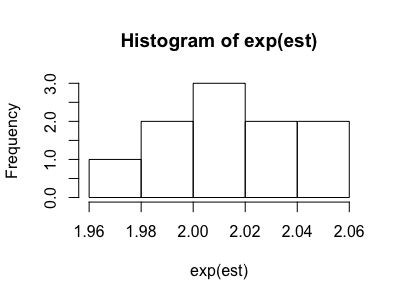
We can run the analysis using different values of the bias parameters. When we use the known, correct values for the bias parameters that we obtained earlier, we obtain OR_YX = 2.03, representing the bias-adjusted effect estimate we expect based on the derivation of the data.

# weighting
set.seed(1234)
adjusted_results_wgt <- adjust_uc_wgt_loop(
  coef_0 = coef(u_model)[1],
  coef_x = coef(u_model)[2],
  coef_c = coef(u_model)[3],
  coef_y = coef(u_model)[4],
  nreps = 10
)

adjusted_results_wgt$estimate # 2.03
adjusted_results_wgt$ci # 1.98, 2.07

# imputation
set.seed(1234)
adjusted_results_imp <- adjust_uc_imp_loop(
  coef_0 = coef(u_model)[1],
  coef_x = coef(u_model)[2],
  coef_c = coef(u_model)[3],
  coef_y = coef(u_model)[4],
  nreps = 10
)

adjusted_results_imp$estimate # 2.03
adjusted_results_imp$ci # 1.95, 2.10

The output can also include a histogram showing the distribution of the OR_YX estimates from each bootstrap sample. We can analyze this plot to see how well the odds ratios converge.

uc_demo_hist

If instead we use bias parameters that are each double the correct value, we obtain OR_YX = 0.81 (0.79, 0.82), an incorrect estimate of effect.

set.seed(1234)
incorrect_results <- adjust_uc_wgt_loop(
  coef_0 = coef(u_model)[1] * 2,
  coef_x = coef(u_model)[2] * 2,
  coef_c = coef(u_model)[3] * 2,
  coef_y = coef(u_model)[4] * 2,
  nreps = 10
)

incorrect_results$estimate # 0.81
incorrect_results$ci # 0.79, 0.82